Curve fitting using numericalnim
Curve fitting is the task of finding the "best" parameters for a given function,
such that it minimizes the error on the given data. The simplest example being,
finding the slope and intersection of a line $y = ax + b$ using such that it minimizes the squared errors
between the data points and the line.
numericalnim implements the Levenberg-Marquardt algorithm(levmarq)
for solving non-linear least squares problems. One such problem is curve fitting, which aims to find the parameters that (locally) minimizes
the error between the data and the fitted curve.
The required imports are:
import numericalnim, ggplotnim, arraymancer, std / [math, sequtils]In some cases you know the actual form of the function you want to fit, but in other cases you may have to guess and try multiple different ones. In this tutorial we will assume we know the form but it works the same regardless. The test curve we will sample points from is $$f(t) = \alpha + \sin(\beta t + \gamma) e^{-\delta t}$$ with $\alpha = 0.5, \beta = 6, \gamma = 0.1, \delta = 1$. This will be a decaying sine wave with an offset. We will add a bit of noise to it as well:
proc f(alpha, beta, gamma, delta, t: float): float =
  alpha + sin(beta * t + gamma) * exp(-delta*t)

let
  alpha = 0.5
  beta = 6.0
  gamma = 0.1
  delta = 1.0
let t = arraymancer.linspace(0.0, 3.0, 20)
let yClean = t.map_inline:
  f(alpha, beta, gamma, delta, x)
let noise = 0.025
let y = yClean + randomNormalTensor(t.shape[0], 0.0, noise)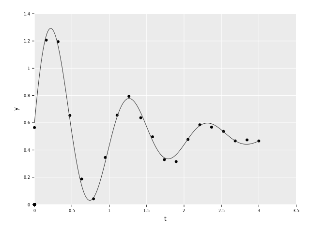
Here we have the original function along with the sampled points with noise.
Now we have to create a proc that levmarq expects. Specifically it
wants all the parameters in a Tensor instead of by themselves:
proc fitFunc(params: Tensor[float], t: float): float =
  let alpha = params[0]
  let beta = params[1]
  let gamma = params[2]
  let delta = params[3]
  result = f(alpha, beta, gamma, delta, t)
As we can see, all the parameters that we want to fit, are passed in as a single 1D Tensor that we unpack for clarity here. The only other thing that is needed is an initial guess of the parameters. We will set them to all 1 here:
let initialGuess = ones[float](4)Now we are ready to do the actual fitting:
let solution = levmarq(fitFunc, initialGuess, t, y)
echo solution
Tensor[system.float] of shape "[4]" on backend "Cpu"
0.503366 6.03074 0.0489922 1.00508
As we can see, the found parameters are very close to the actual ones. But maybe we can do better,
levmarq accepts an options parameter which is the same as the one described in Optimization
with the addition of the lambda0 parameter. We can reduce the tol and see if we get an even better fit:
let options = levmarqOptions(tol=1e-10)
let solution = levmarq(fitFunc, initialGuess, t, y, options=options)
echo solution
Tensor[system.float] of shape "[4]" on backend "Cpu"
0.503366 6.03074 0.0489921 1.00508
As we can see, there isn't really any difference. So we can conclude that the found solution has in fact converged.
Here's a plot comparing the fitted and original function:
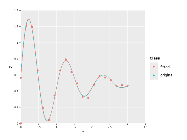
As we can see, the fitted curve is quite close to the original one.
Errors & Uncertainties
We might also want to quantify exactly how good of a fit the computed weights give. One measure commonly used is $\chi^2$: $$\chi^2 = \sum_i \frac{(y_i - \hat{y}(x_i))^2}{\sigma_i^2}$$ where $y_i$ and $x_i$ are the measurements, $\hat{y}$ is the fitted curve and $\sigma_i$ is the standard deviation (uncertainty/error) of each of the measurements. We will use the noise size we used when generating the samples here, but in general you will have to figure out yourself what errors are in your situation. It may for example be the resolution of your measurements or you may have to approximate it using the data itself.
We now create the error vector and sample the fitted curve:
let yError = ones_like(y) * noise
let yCurve = t.map_inline:
  fitFunc(solution, x)
Now we can calculate the $\chi^2$ using numericalnim's chi2 proc:
let chi = chi2(y, yCurve, yError)
echo "χ² = ", chi
χ² = 16.93637503832095
Great! Now we have a measure of how good the fit is, but what if we add more points? Then we will get a better fit, but we will also get more points to sum over. And what if we choose another curve to fit with more parameters? Then we may be able to get a better fit but we risk overfitting. Reduced $\chi^2$ is a measure which adjusts $\chi^2$ to take these factors into account. The formula is: $$\chi^2_{\nu} = \frac{\chi^2}{n_{\text{obs}} - m_{\text{params}}}$$ where $n_{\text{obs}}$ is the number of observations and $m_{\text{params}}$ is the number of parameters in the curve. The difference between them is denoted the degrees of freedom (dof). This is simplified, the mean $\chi^2$ score adjusted to penalize too complex curves.
Let's calculate it!
let reducedChi = chi / (y.len - solution.len).float
echo "Reduced χ² = ", reducedChi
Reduced χ² = 1.058523439895059
As a rule of thumb, values around 1 are desirable. If it is much larger than 1, it indicates a bad fit. And if it is much smaller than 1 it means that the fit is much better than the uncertainties suggested. This could either mean that it has overfitted or that the errors were overestimated.
Parameter uncertainties
To find the uncertainties of the fitted parameters, we have to calculate
the covariance matrix:
$$\Sigma = \sigma^2 H^{-1}$$
where $\sigma^2$ is the standard deviation of the residuals and $H$ is
the Hessian of the objective function (we used $\chi^2$).
numericalnim can compute the covariance matrix for us using paramUncertainties:
let cov = paramUncertainties(solution, fitFunc, t, y, yError, returnFullCov=true)
echo cov
Tensor[system.float] of shape "[4, 4]" on backend "Cpu" |1.70541e-05 1.58002e-05 -1.04688e-05 -2.4089e-06| |1.58002e-05 0.000707119 -0.000250193 -9.67158e-06| |-1.04688e-05 -0.000250193 0.000245993 4.47236e-06| |-2.4089e-06 -9.67158e-06 4.47236e-06 0.000446313|
That is the full covariance matrix, but we are only interested in the diagonal elements.
By default returnFullCov is false and then we get a 1D Tensor with the diagonal instead:
let variances = paramUncertainties(solution, fitFunc, t, y, yError)
echo variances
Tensor[system.float] of shape "[4]" on backend "Cpu"
1.70541e-05 0.000707119 0.000245993 0.000446313
It's important to note that these values are the variances of the parameters. So if we want the standard deviations we will have to take the square root:
let paramUncertainty = sqrt(variances)
echo "Uncertainties: ", paramUncertainty
Uncertainties: Tensor[system.float] of shape "[4]" on backend "Cpu"
0.00412966 0.0265917 0.0156842 0.0211261
All in all, these are the values and uncertainties we got for each of the parameters:
echo "α = ", solution[0], " ± ", paramUncertainty[0]
echo "β = ", solution[1], " ± ", paramUncertainty[1]
echo "γ = ", solution[2], " ± ", paramUncertainty[2]
echo "δ = ", solution[3], " ± ", paramUncertainty[3]
α = 0.5033663155477502 ± 0.004129656819321223 β = 6.030735258169046 ± 0.02659170150059456 γ = 0.0489920969605781 ± 0.01568416864219338 δ = 1.005076206375797 ± 0.02112613290725861