Optimize functions in Nim
Optimization is a common task, you have a function, $f(\theta)$ and would like to find the parameters, $\theta_{\text{min}}$, that either minimize or maximize the function. We will use numericalnim in this tutorial to minimize the Rosenbrock banana 🍌 function:
$$f(x, y) = (1 - x)^2 + 100(y - x^2)^2$$
It looks like this with its minimum at $(x, y) = (1, 1)$:
import ggplotnim, numericalnim, benchy, std / [math]let (x, y) = meshgridFlat(linspace(-2.0, 2.0, 100).toTensor, linspace(-1.0, 3.0, 100).toTensor)
# Log z to reduce its range
let z = log10((1.0 -. x) ^. 2 + 100.0 * (y - x ^. 2) ^. 2)
let df = toDf(x, y, z)
ggplot(df, aes("x", "y", fill="z")) +
geom_raster() +
ggsave("images/banana_function.png")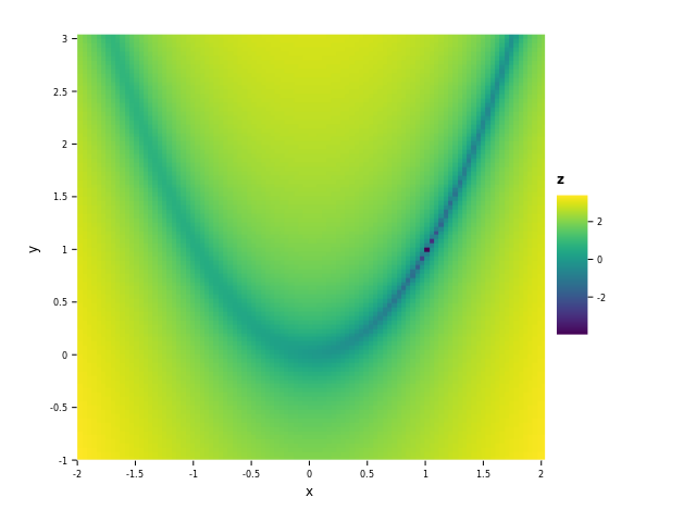
As you can see the function's shape resembles a banana, and the dark spot
on the right-hand side is the minimum. The format that numericalnim expects of the function is:
proc f(theta: Tensor[float]): float =
  let x = theta[0]
  let y = theta[1]
  (1.0 - x) ^ 2 + 100.0 * (y - x ^ 2) ^ 2
where theta is a vector containing all the input arguments, x and y in this case.
The optimization methods numericalnim offers are:
Now we are ready to try out the different methods, the only thing we need to provide is a start guess. To make it a bit of a challenge, let us start on the other side of the hill at $(-0.5, 2)$.
let theta0 = [-0.5, 2.0].toTensor()
let solutionSteepest = steepestDescent(f, theta0)
echo "Steepest: ", solutionSteepest
let solutionNewton = newton(f, theta0)
echo "Newton: ", solutionNewton
let solutionBfgs = bfgs(f, theta0)
echo "BFGS: ", solutionBfgs
let solutionLbfgs = lbfgs(f, theta0)
echo "LBFGS: ", solutionLbfgs

benchy.timeIt "Steepest":
  keep steepestDescent(f, theta0)
benchy.timeIt "Newton":
  keep newton(f, theta0)
benchy.timeIt "BFGS":
  keep bfgs(f, theta0)
benchy.timeIt "LBFGS":
  keep lbfgs(f, theta0)
Steepest: Tensor[system.float] of shape "[2]" on backend "Cpu"
0.99157 0.983176
Newton: Tensor[system.float] of shape "[2]" on backend "Cpu"
1 1
BFGS: Tensor[system.float] of shape "[2]" on backend "Cpu"
1 1
LBFGS: Tensor[system.float] of shape "[2]" on backend "Cpu"
1 1
min time avg time std dv runs name
158.509 ms 325.429 ms ±106.262 x16 Steepest
0.207 ms 0.235 ms ±0.012 x1000 Newton
2.216 ms 3.286 ms ±0.601 x1000 BFGS
3.784 ms 4.218 ms ±0.760 x1000 LBFGS
As we can see, Newton, BFGS and LBFGS found the exact solution and they did it fast. Steepest descent didn't find as good a solution and took by far the longest time. Steepest descent has an order of convergence of $O(N)$, Newton has $O(N^2)$ and (L)BFGS has one somewhere in-between. So typically Newton will require the least amount of steps. But it also has the most expensive step to perform. For a small problem like this, it is not a problem, but say that you have more than a thousand variables in $\theta$, then it will start to become slow. Typically LBFGS is a good trade-off between number of steps and the time per step.
Analytical gradient
In the example above we did not provide an analytical gradient, so instead numerical gradients was calculated.
This is typically slower than providing the gradient as a function as f has to be called multiple times
and the steps are not as accurate. All the above-mentioned methods supports this.
To supply a analytical gradient is to create a function of the following form:
proc fGradient(theta: Tensor[float]): Tensor[float] =
  let x = theta[0]
  let y = theta[1]
  result = newTensor[float](2)
  result[0] = -2 * (1 - x) + 100 * 2 * (y - x*x) * -2 * x
  result[1] = 100 * 2 * (y - x*x)
It takes the parameters as input and returns a Tensor of the same size with the gradient with respect to each parameter. It can then be supplied like this:
let theta0 = [-0.5, 2.0].toTensor()
let solutionLbfgs = lbfgs(f, theta0, analyticGradient=fGradient)
echo "LBFGS (analytic): ", solutionLbfgs
LBFGS (analytic): Tensor[system.float] of shape "[2]" on backend "Cpu"
1 1
No surprise that it also managed to find the correct solution.
Options
There are several options you can provide to the solver. Here's a summary of some of them:
tol: The error tolerance for when to stop.alpha: The step size to use.fastMode: Use a lower-order approximation of the derivatives to exchange accuracy for speed.maxIterations: The maximum number of iterations to run the solver for until stopping.lineSearchCriterion: Different methods of linesearch (Armijo, Wolfe, WolfeStrong, NoLineSearch).
These are provided by creating a options object. Each method has its own initializer, for example:
let theta0 = [-0.5, 2.0].toTensor()

let steepestOption = steepestDescentOptions[float](alpha=1e-3, fastMode=true)
let steepestSolution = steepestDescent(f, theta0, options=steepestOption)

let lbfgsOption = lbfgsOptions[float](lineSearchCriterion=Wolfe)
let lbfgsSolution = lbfgs(f, theta0, options=lbfgsOption)
Further reading
- numericalnim's documentation on optimization
- We also have an article on curve fitting which allows you to optimize parameters to minimize the error between a curve and data points.