1D Numerical Integration
In this tutorial you will learn learn how to use numericalnim to perform numerical integration both on discrete data and continuous functions.
Integrate Continuous Functions
We will start off by integrating some continuous function using a variety of methods and comparing their accuracies and performances so that you can make an educated choice of method. Let's start off with creating the data to integrate, I have choosen to use the humps function from MATLAB's demos:
$$ f(x) = \frac{1}{(x - 0.3)^2 + 0.01} + \frac{1}{(x - 0.9)^2 + 0.04} - 6 $$
It has the primitive function:
$$ F(x) = 10 \arctan(10x - 3) + 5 \arctan\left(5x - \frac{9}{2}\right) - 6x $$
Let's code them!
import math, sequtils
import numericalnim, ggplotnim, benchy
proc f(x: float, ctx: NumContext[float, float]): float =
  result = 1 / ((x - 0.3)^2 + 0.01) + 1 / ((x - 0.9)^2 + 0.04) - 6

proc F(x: float): float =
  result = 10*arctan(10*x-3) + 5*arctan(5*x - 9/2) - 6*x
As you can see, we defined f not as just proc f(x: float): float but added a ctx: NumContext[float, float] as well.
That is because numericalnim's integration methods expect a proc with the signature proc f[T; U](x: U, ctx: NumContext[T, U]): T,
where U is the type used for computations internally (typically a float or a type like it) and T is the user defined
type that is the result of the function to be integrated (and may be used to include custom data in the body of the function).
This means that you can both integrate functions returning other types than float, namely T if they provide a certain
set of supported operations, as well as perform the integration using types U as long as they behave "float-like".
We won't be integrating F (it is the indefinite integral already) so I skipped adding ctx there for simplicity.
Aren't you curious of what f(x) looks like? Thought so! Let's plot them using ggplotnim,
a more detailed plotting tutorial can be found here.
let ctxPlot = newNumContext[float, float]()
let xPlot = numericalnim.linspace(0, 1, 1000)
let yPlot = xPlot.mapIt(f(it, ctxPlot))

let dfPlot = toDf(xPlot, yPlot)
ggplot(dfPlot, aes("xPlot", "yPlot")) +
  geom_line() +
  ggsave("images/humps.png")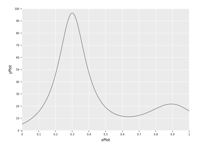
Let the integration begin!
Now we have everything we need to start integrating. The specific integral we want to compute is:
$$ \int_0^1 f(x), \mathrm{d}x $$
The methods we will use are: trapz(link), simpson(link),
gaussQuad(link), romberg(link), adaptiveSimpson and adaptiveGauss.
Where the last three are adaptive methods and the others are fixed-step methods. We will use a tolerance tol=1e-6
for the adaptive methods and N=100 intervals for the fixed-step methods.
Let's code this now and compare them!
let a = 0.0
let b = 1.0
let tol = 1e-6
let N = 100
let exactIntegral = F(b) - F(a)

let trapzError = abs(trapz(f, a, b, N) - exactIntegral)
let simpsonError = abs(simpson(f, a, b, N) - exactIntegral)
let gaussQuadError = abs(gaussQuad(f, a, b, N) - exactIntegral)
let rombergError = abs(romberg(f, a, b, tol=tol) - exactIntegral)
let adaptiveSimpsonError = abs(adaptiveSimpson(f, a, b, tol=tol) - exactIntegral)
let adaptiveGaussError = abs(adaptiveGauss(f, a, b, tol=tol) - exactIntegral)

echo "Trapz Error:      ", trapzError
echo "Simpson Error:    ", simpsonError
echo "GaussQuad Error:  ", gaussQuadError
echo "Romberg Error:    ", rombergError
echo "AdaSimpson Error: ", adaptiveSimpsonError
echo "AdaGauss Error:   ", adaptiveGaussError
Trapz Error: 0.00123417243757018 Simpson Error: 3.129097940757219e-07 GaussQuad Error: 3.907985046680551e-14 Romberg Error: 3.411159354982374e-09 AdaSimpson Error: 1.061664534063311e-09 AdaGauss Error: 0.0
It seems like the gauss methods were the most accurate with Romberg and Simpson
coming afterwards and in last place trapz. But at what cost did these scores come at? Which method was the fastest?
Let's find out with a package called benchy. keep is used to prevent the compiler from optimizing away the code:
timeIt "Trapz":
  keep trapz(f, a, b, N)

timeIt "Simpson":
  keep simpson(f, a, b, N)

timeIt "GaussQuad":
  keep gaussQuad(f, a, b, N)

timeIt "Romberg":
  keep romberg(f, a, b, tol=tol)

timeIt "AdaSimpson":
  keep adaptiveSimpson(f, a, b, tol=tol)

timeIt "AdaGauss":
  keep adaptiveGauss(f, a, b, tol=tol)
min time avg time std dv runs name 0.015 ms 0.017 ms ±0.001 x1000 Trapz 0.016 ms 0.019 ms ±0.064 x1000 Simpson 0.065 ms 0.073 ms ±0.093 x1000 GaussQuad 0.035 ms 0.038 ms ±0.002 x1000 Romberg 0.293 ms 0.605 ms ±1.541 x1000 AdaSimpson 0.032 ms 0.037 ms ±0.040 x1000 AdaGauss
As we can see, all methods except AdaSimpson were roughly equally fast. So if I were to choose
a winner, it would be adaptiveGauss because it was the most accurate while still being among
the fastest methods.
Cumulative Integration
There is one more type of integration one can do, namely cumulative integration. This is for the case
when you don't just want to calculate the total integral but want an approximation for F(X), so we
need the integral evaluated at multiple points. An example is if we have the acceleration a(t) as a function.
If we integrate it we get the velocity, but to be able to integrate the velocity (to get the distance)
we need it as a function, not a single value. That is where cumulative integration comes in!
The methods available to us from numericalnim are: cumtrapz, cumsimpson, cumGauss and cumGaussSpline.
All methods except cumGaussSpline returns the cumulative integral as a seq[T], but this instead returns a
Hermite spline. We will both be calculating the errors and visualizing the different approximations of F(x).
Let's get coding!
let a = 0.0
let b = 1.0
let tol = 1e-6
let N = 100
let dx = (b - a) / N.toFloat
let x = numericalnim.linspace(a, b, 100)
var exact = x.mapIt(F(it) - F(a))
let yTrapz = cumtrapz(f, x, dx=dx)
let ySimpson = cumsimpson(f, x, dx=dx)
let yGauss = cumGauss(f, x, tol=tol, initialPoints=x)
echo "Trapz Error: ", sum(abs(exact.toTensor - yTrapz.toTensor))
echo "Simpson Error: ", sum(abs(exact.toTensor - ySimpson.toTensor))
echo "Gauss Error: ", sum(abs(exact.toTensor - yGauss.toTensor))
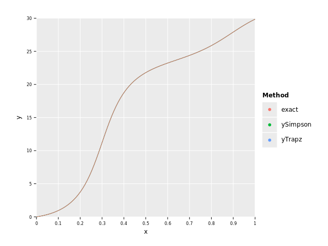
let df = toDf(x, exact, yTrapz, ySimpson, yGauss)
# Rewrite df in long format for plotting
let dfLong = df.gather(["exact", "yTrapz", "ySimpson", "yGauss"], key="Method", value="y")
ggplot(dfLong, aes("x", "y", color="Method")) +
geom_line() +
ggsave("images/continuousHumpsComparaision.png")Trapz Error: 0.1629684871013665 Simpson Error: 0.001052250314251719 Gauss Error: 5.453207330141652e-13
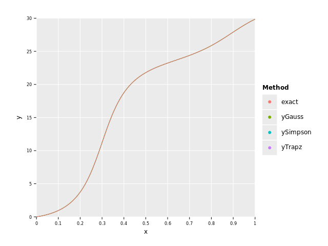
As we can see in the graph they are all so close to the exact curve that you can't distingush between them, but when we look at the total error we see that once again the Gauss method is superior.
Note:
When we called
cumGausswe passed in a parameterinitialPointsas well. The reason for that is the fact that the Gauss method uses polynomials of degree 21 in its internal calculations while the final interpolation at the x-values inxis performed using a 3rd degree polynomial. This means that Gauss internally might only need quite few points because of its high degree, but that means we get too few points for the final 3rd degree interpolation. So to make sure we have enough points in the end we supply it with enough initial points so that it has enough points to make good predictions even if it doesn't split any additional intervals. By default it uses 100 equally spaced points though so unless you know you need far more or less points you should be good. This is especially important when usingcumGaussSplineas we need enough points to construct an accurate spline.
The last method is cumGaussSpline which is identical to cumGauss except it constructs a Hermite spline
from the returned values which can be evaluated when needed.
let a = 0.0
let b = 1.0
let tol = 1e-6

let spline = cumGaussSpline(f, a, b, tol=tol)

echo "One point: ", spline.eval(0.0) # evaluate it in a single point
echo "Three points: ", spline.eval(@[0.0, 0.5, 1.0]) # or multiple at once

# Thanks to converter you can integrate a spline by passing it as the function:
echo "Integrate it again: ", adaptiveGauss(spline, a, b)
One point: 0.0 Three points: @[0.0, 21.78684367031352, 29.85832539549869] Integrate it again: 17.26538964301353
I think that about wraps it up regarding integrating continuous functions! Let's take a look at integrating discrete data now!
Integrate Discrete Data
Discrete data is a different beast than continuous functions as we have limited data. Therefore, the choice
of integration method is even more important as we can't exchange performance to get more accurate results
like we can with continuous functions (we can increase the number of intervals for example). So we want to make the
most out of the data we have, and any knowledge we have about the nature of the data is helpful.
For example if we know the data isn't smooth (discontinuities), then trapz could be a better choice
than let's say simpson, because simpson assumes the data is smooth.
Let's sample f(x) from above at let's say 9 points and plot how much information we lose by
plotting the sampled points, a Hermite Spline interpolation of them and the original function:
var xSample = numericalnim.linspace(0.0, 1.0, 9)
var ySample = xSample.mapIt(f(it, nil)) # nil can be passed in instead of ctx if we don't use it

let xDense = numericalnim.linspace(0, 1, 1000) # "continuous" x
let yDense = xDense.mapIt(f(it, nil))

var sampledSpline = newHermiteSpline(xSample, ySample)
var ySpline = sampledSpline.eval(xDense)

var dfSample = toDf(xSample, ySample, xDense, yDense, ySpline)
ggplot(dfSample) +
  #geom_point(data = dfSample.filter(f{Value -> bool: not `xSample`.isNull.toBool}), aes = aes("xSample", "ySample", color = "Sampled")) +
  geom_point(aes("xSample", "ySample", color="Sampled")) +
  geom_line(aes("xDense", "ySpline", color="Sampled")) +
  geom_line(aes("xDense", "yDense", color="Dense")) +
  scale_x_continuous() + scale_y_continuous() +
  ggsave("images/sampledHumps.png")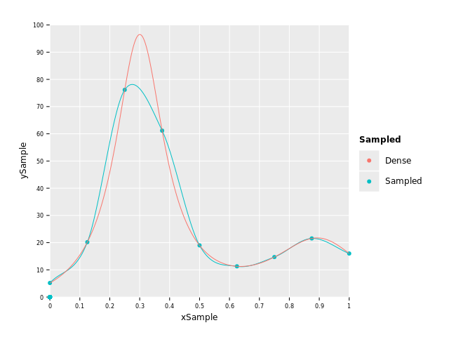
As you can see, the resolution was too small to fully account for the big peak and undershoots it by quite a margin. Without having known the "real" function in this case we wouldn't have known this of course, and that is most often the case when we have discrete data. Therefore, the resolution of the data is crucial for the accuracy. But let's say this is all the data we have at our disposal and let's see how the different methods perform.
The integration methods at our disposal are:
trapz: Works for any data.simpson: Works for any data with 3 or more data points.romberg: Works only for equally spaced points. The number of points must also be of the form2^n + 1(eg. 3, 5, 9, 17, 33 etc).
Luckily for us our data satisfies all of them ;) So let's get coding:
let exact = F(1) - F(0)

var trapzIntegral = trapz(ySample, xSample)
var simpsonIntegral = simpson(ySample, xSample)
var rombergIntegral = romberg(ySample, xSample)

echo "Exact:   ", exact
echo "Trapz:   ", trapzIntegral
echo "Simpson: ", simpsonIntegral
echo "Romberg: ", rombergIntegral
echo "Trapz Error:   ", abs(trapzIntegral - exact)
echo "Simpson Error: ", abs(simpsonIntegral - exact)
echo "Romberg Error: ", abs(rombergIntegral - exact)
Exact: 29.85832539549867 Trapz: 29.33117732440506 Simpson: 29.07021311510501 Romberg: 28.53591179962037 Trapz Error: 0.5271480710936096 Simpson Error: 0.788112280393662 Romberg Error: 1.322413595878309
As expected all the methods underestimated the integral, but it might be unexpected that
trapz performed the best out of them. Let's add a few more points, why not 33, and let's see if
that changes things!
xSample = numericalnim.linspace(0.0, 1.0, 33)
ySample = xSample.mapIt(f(it, nil))

sampledSpline = newHermiteSpline(xSample, ySample)
ySpline = sampledSpline.eval(xDense)

dfSample = toDf(xSample, ySample, xDense, yDense, ySpline)
ggplot(dfSample) +
  geom_point(aes("xSample", "ySample", color="Sampled")) +
  geom_line(aes("xDense", "ySpline", color="Sampled")) +
  geom_line(aes("xDense", "yDense", color="Dense")) +
  scale_x_continuous() + scale_y_continuous() +
  ggsave("images/sampledHumps33.png")

trapzIntegral = trapz(ySample, xSample)
simpsonIntegral = simpson(ySample, xSample)
rombergIntegral = romberg(ySample, xSample)

echo "Exact:   ", exact
echo "Trapz:   ", trapzIntegral
echo "Simpson: ", simpsonIntegral
echo "Romberg: ", rombergIntegral
echo "Trapz Error:   ", abs(trapzIntegral - exact)
echo "Simpson Error: ", abs(simpsonIntegral - exact)
echo "Romberg Error: ", abs(rombergIntegral - exact)
Exact: 29.85832539549867 Trapz: 29.84626609518119 Simpson: 29.85807788992319 Romberg: 29.84669883230159 Trapz Error: 0.01205930031748892 Simpson Error: 0.0002475055754800337 Romberg Error: 0.01162656319708333
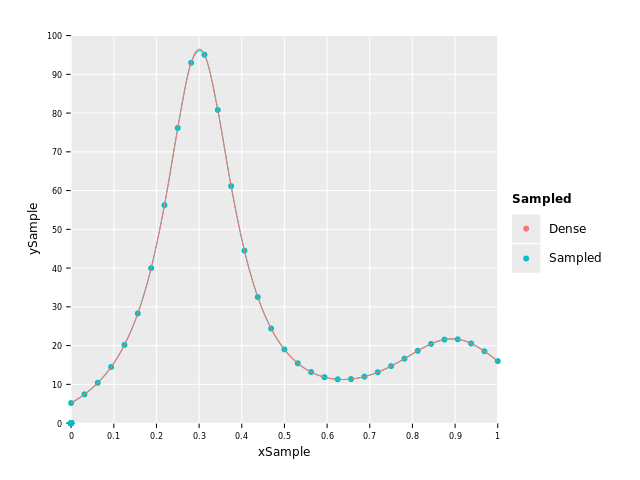
As expected all methods became more accurate when we increased the amount of points.
And from the graph we can see that the points capture the shape of the curve much better now.
We can also note that simpson has overtaken trapz and romberg is neck-in-neck with trapz now.
Experiment for yourself with different number of points, but asymptotically romberg will eventually
beat simpson when enough points are used.
The take-away from this very limited testing is that depending on the characteristics and quality
of the data, different methods might give the most accurate answer. Which one is hard to tell in general
but trapz might be more robust for very sparse data as it doesn't "guess" as much as the others. But once again,
it entirely depends on the data, so make sure to understand your data!
Cumulative Integration with Discrete Data
Performing cumulative integration on discrete data works the same as for continuous functions. The only differences are that
only cumtrapz and cumsimpson are available and that you pass in y and x instead of f:
let a = 0.0
let b = 1.0
let tol = 1e-6
let N = 100

let x = numericalnim.linspace(a, b, N)
let y = x.mapIt(f(it, nil))
var exact = x.mapIt(F(it) - F(a))

let yTrapz = cumtrapz(y, x)
let ySimpson = cumsimpson(y, x)

echo "Trapz Error:   ", sum(abs(exact.toTensor - yTrapz.toTensor))
echo "Simpson Error: ", sum(abs(exact.toTensor - ySimpson.toTensor))

let df = toDf(x, exact, yTrapz, ySimpson)
# Rewrite df in long format for plotting
let dfLong = df.gather(["exact", "yTrapz", "ySimpson"], key="Method", value="y")
ggplot(dfLong, aes("x", "y", color="Method")) +
  geom_line() +
  ggsave("images/discreteHumpsComparaision.png")
Trapz Error: 0.1667713445258438 Simpson Error: 0.001344104336917881