Solve ordinary differential equations in Nim

Ordinary differential equations (ODEs) describe so many aspects of nature, but many of them do not have simple solutions you can solve using pen and paper. That is where numerical solutions come in. They allow us to solve these equations approximately. We will use numericalnim for this. The required imports are:

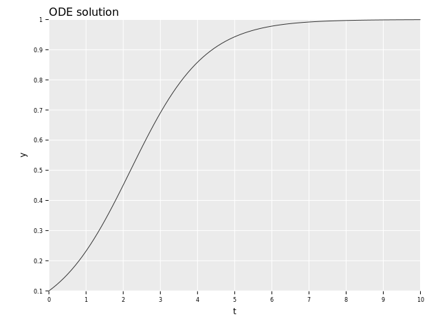
import ggplotnim, numericalnim, benchy, std / [math, sequtils]

We will use an ODE with a known solution to be able to compare our numerical solution with the analytical one. The ODE we will solve is: $$y' = y (1 - y)$$ $$y(0) = 0.1$$ which has the solution of a sigmoid: $$y(t) = \frac{1}{1 + 9 e^{-t}}$$

This equation can for example describe a system which grows exponentially at the beginning, but due to limited amounts of resources the growth stops and it reaches an equilibrium. The solution looks like this:

Let's code

Let us create the function for evaluating the derivative $y'(t, y)$:

proc exact(t: float): float =
  1 / (1 + 9*exp(-t))

proc dy(t: float, y: float, ctx: NumContext[float, float]): float =
  y * (1 - y)

numericalnim expects a function of the form proc(t: float, y: T, ctx: NumContext[T, float]): T, where T is the type of the function value (can be Tensor[float] if you have a vector-valued function), and ctx is a context variable that allows you to pass parameters or save information between function calls. Now we need to define a few parameters before we can do the actual solving:

let t0 = 0.0
let tEnd = 10.0
let y0 = 0.1 # initial condition
let tspan = linspace(t0, tEnd, 20)
let odeOptions = newODEoptions(tStart = t0)

Here we define the starting time (t0), the value of the function at that time (y0), the time points we want to get the solution at (tspan) and the options we want the solver to use (odeOptions). There are more options you can pass, for example the timestep dt used for fixed step-size methods and dtMax and dtMin used by adaptive methods. The only thing left is to choose which method we want to use. The fixed step-size methods are:

• heun2
• ralston2
• kutta3
• heun3
• ralston3
• ssprk3
• ralston4
• kutta4
• rk4

And the adaptive methods are:

• rk21
• bs32
• dopri54
• tsit54
• vern65

That is a lot to choose from, but its hard to go wrong with any of the adaptive methods dopri54, tsit54 & vern65. So let's use tsit54!

let (t, y) = solveOde(dy, y0, tspan, odeOptions, integrator="tsit54")
let error = abs(y[^1] - exact(t[^1]))
echo "Error: ", error

Error: 3.33066907387547e-16

We call solveOde with our parameters and it returns one seq with our time points and one with our solution at those points. We can check the error at the last point and we see that it is around 3e-16. Let's plot this solution:

let yExact = t.mapIt(exact(it))
var df = toDf(t, y, yExact)
df = df.gather(["y", "yExact"], key="Class", value="y")
ggplot(df, aes("t", "y", color="Class")) +
  geom_line() +
  ggtitle("Tsit54 Solution") +
  ggsave("images/tsit54_solution.png")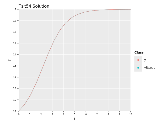

As we can see, the graphs are very similar so it seems to work :D.

Now you might be curios how well a few of the other methods performed, and here you have it:

• heun2: 4.961920e-12

• rk4: 2.442491e-15

• rk21: 4.990390e-08

• tsit54: 3.330669e-16

We can see that the higher-order methods has a lower error compared to the lower-order ones. Tweaking the odeOptions would probably get them on-par with the others. There is one parameter we haven't talked about though, the execution time. Let's look at that and see if it bring any further insights:

   min time    avg time  std dv   runs name
  11.259 ms   20.406 ms  ±6.787   x243 heun2
  14.426 ms   16.404 ms  ±3.768   x295 rk4
   0.259 ms    0.284 ms  ±0.009  x1000 rk21
   0.304 ms    0.361 ms  ±0.118  x1000 tsit54

As we can see, the adaptive methods are orders of magnitude faster while achieving roughly the same errors. This is because they take fewer and longer steps when the function is flatter and only decrease the step-size when the function is changing more rapidly.

Vector-valued functions

Now let us look at another example which is a simplified version of what you might get from discretizing a PDE, multiple function values. The equation in question is $$y'' = -y$$ $$y(0) = 0$$ $$y'(0) = 1$$ This has the simple solution $$y(t) = \sin(t)$$ but it is not on the form y' = ... that numericalnim wants, so we have to rewrite it. We introduce a new variable $z = y'$ and then we can rewrite the equation like: $$y'' = (y')' = z' = -y$$ This gives us a system of ODEs: $$y' = z$$ $$z' = -y$$ $$y(0) = 0$$ $$z(0) = y'(0) = 1$$

This can be written in vector-form to simplify it: $$\mathbf{v} = [y, z]^T$$ $$\mathbf{v}' = [z, -y]^T$$ $$\mathbf{v}(0) = [0, 1]^T$$

Now we can write a function which takes as input a $\mathbf{v}$ and returns the derivative of them. This function can be represented as a matrix multiplication, $\mathbf{v}' = A\mathbf{v}$, with a matrix $A$: $$A = \begin{bmatrix}0 & 1\\-1 & 0\end{bmatrix}$$

Let us code this function but let us also take this opportunity to explore the NumContext to pass in A.

proc dv(t: float, y: Tensor[float], ctx: NumContext[Tensor[float], float]): Tensor[float] =
  ctx.tValues["A"] * y

NumContext consists of two tables, ctx.fValues which can contain floats and ctx.tValues which in this case can hold Tensor[float]. So we access A which we will insert when creating the context variable:

var ctx = newNumContext[Tensor[float], float]()
ctx.tValues["A"] = @[@[0.0, 1.0], @[-1.0, 0.0]].toTensor

Now we are ready to setup and run the simulation as we did previously:

let t0 = 0.0
let tEnd = 20.0
let y0 = @[@[0.0], @[1.0]].toTensor # initial condition
let tspan = linspace(t0, tEnd, 50)
let odeOptions = newODEoptions(tStart = t0)

let (t, y) = solveOde(dv, y0, tspan, odeOptions, ctx=ctx, integrator="tsit54")
let yEnd = y[^1][0, 0]
let error = abs(yEnd - sin(tEnd))
echo "Error: ", error

Error: 2.114974861910923e-13

The error is nice and low. The error for the other methods are along with the timings:

• heun2: 1.361859e-08

• rk4: 1.357736e-11

• rk21: 1.381992e-04

• tsit54: 2.114975e-13

2615.167 ms 2626.198 ms ±15.601     x2 heun2
5261.133 ms 5261.133 ms  ±0.000     x1 rk4
  50.778 ms   51.349 ms  ±0.291    x98 rk21
 224.308 ms  225.149 ms  ±0.704    x23 tsit54

We can once again see that the high-order adaptive methods are both more accurate and faster than the fixed-order ones.

Further reading

• numericalnim's documentation on ODEs