Interpolate discrete data in Nim
Very seldom when dealing with real data do you have an exact function you can evaluate at any point you would like. Often you have data in a finite number of discrete points instead. Two common ways to solve this problem is to either interpolate the data or if you know the form it should take you can do curve fitting. In this tutorial we will cover the interpolation approach in 1D, 2D and 3D for some cases.
We will be using numericalnim for this and the imports we will need are:
import numericalnim, arraymancer, ggplotnim, std/[math, sequtils]1D Interpolation
This is the simplest case of interpolation and numericalnim can handle both evenly spaced and variable spacing in 1D.
We will use the function $$f(x) = \sin(3x) (x-2)^2$$ for our benchmarks:
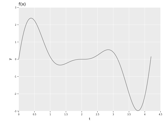
Let's get interpolating! We first define the function and sample from it:
proc f(x: float): float = sin(3*x) * (x - 2)^2

let x = linspace(0.0, 4.2, 10)
let y = x.map(f)
Now we are ready to create the interpolator! For 1D there are these options available:
- Linear:
newLinear1D - Cubic spline:
newCubicSpline(only supports floats) - Hermite spline:
newHermiteSpline
They all have the same API accepting seqs of x- and y-values.
The Hermite spline can optionally supply the derivatives at each point as well.
We will be using the Hermite spline without the derivatives, they will be approximated
using finite differences for us.
let interp = newHermiteSpline(x, y)Now that we have constructed the interpolator, we can evaluate it using eval.
It accepts either a single input or a seq of inputs:
echo interp.eval(1.0)
echo interp.eval(@[1.0, 2.0])
0.2080277072449881 @[0.2080277072449881, 0.01739123273517499]
We can now evaluate it on a denser set of points and compare it to the original function:
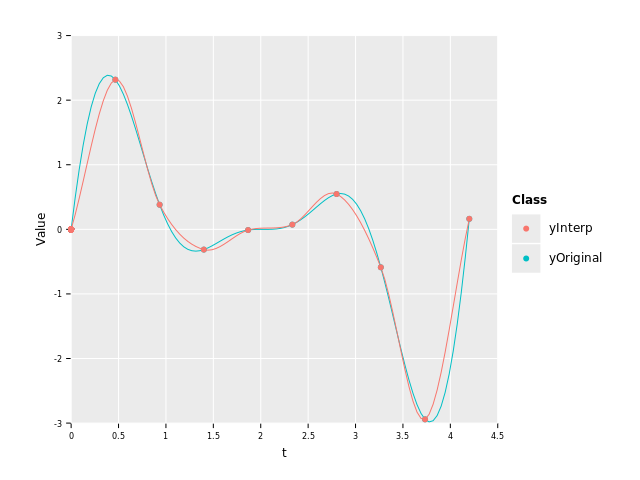
As we can see, the interpolant does a decent job of approximating the function. It is worse where the function is changing a lot and closer to the original in the middle where there is less happening.
Extrapolation
For 1D interpolators, extrapolation is supported. The available methods are:
Constant: Set all points outside the range of the interpolator to a specified value.Edge: Use the value of the left/right edge.Linear: Uses linear extrapolation using the two points closest to the edge.Native(default): Uses the native method of the interpolator to extrapolate. For Linear1D it will be a linear extrapolation, and for Cubic and Hermite splines it will be cubic extrapolation.Error: Raises anValueErrorifxis outside the range.
The extrapolation method is optionally supplied as an argument to eval and derivEval:
echo "Edge: ", interp.eval(-1.0, Edge) # will use the value at x=0
echo "Constant: ", interp.eval(-1.0, Constant, NaN) # will return NaN
echo "Linear: ", interp.eval(-1.0, ExtrapolateKind.Linear)
echo "Native: ", interp.eval(-1.0) # will use Native by default
Edge: 0.0 Constant: nan Linear: -4.964789592037099 Native: 25.7213250632593
As you can see, the choice of extrapolation method affects the values considerably.
Keep in mind though that -1.0 is quite a big extrapolation and the further away we go, the worse the approximation gets.
Here is a visual example of how the different methods behave. I have removed the two outermost points on each side from the example before (ignore the point at (0, 0), it's a bug):
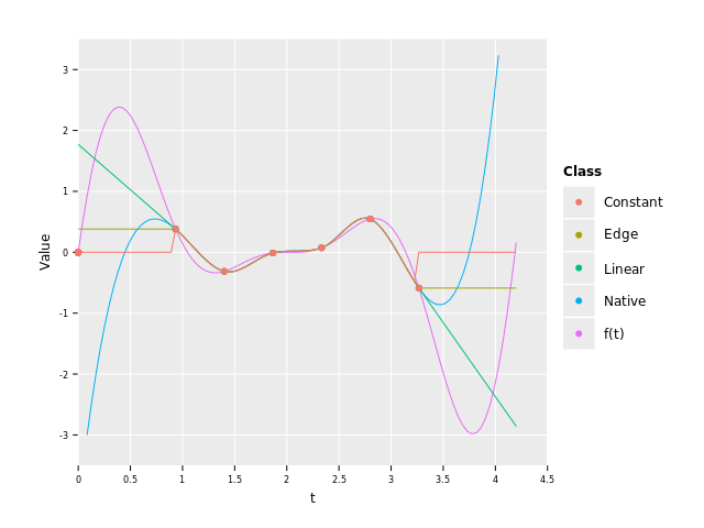
As we can see, the Edge and Constant are just horizontal lines while Linear has the same slope as the edge of the interpolant.
Native on the other hand is smooth but quite quickly starts to take off towards $\pm \infty$ (for the linear interpolator it would behave the same as Linear though).
Which method you should use is very dependent on the application and what behavior you want it to exhibit.
Of course, you should try to avoid extrapolation whenever possible.
2D interpolation
For 2D interpolation, numericalnim offers 3 methods for gridded data:
- Nearest neighbour:
newNearestNeighbour2D - Bilinear:
newBilinearSpline - Bicubic:
newBicubicSpline
and 2 methods for scattered data:
- Barycentric:
newBarycentric2D - Radial basis function:
newRbfThe RBF method isn't unique to 2D and works for any dimension, see the next section for more on that.
For this tutorial, we will focus on the Bicubic spline but NearestNeighbour and Bilinear spline have the same API.
Let's first choose a suitable function to interpolate:
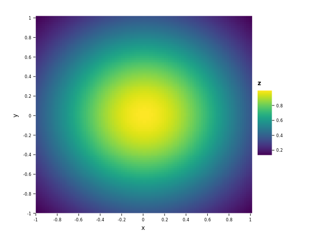
$$f(x, y) = e^{-(x^2 + y^2)}$$
This will be a Gaussian centered around (0, 0), here's a heatmap showing the function:
Now we are ready to sample our function. The inputs expected are the limits in $x$ and $y$ along with the function values in grid as a Tensor. So if we have a 3x3 grid of data points, the Tensor should have shape 3x3 as well. Because the data is known to be on a grid, you don't have to give all the points on it, it's enough to only provide the limits as two tuples.
proc f(x, y: float): float =
  exp(-(x*x + y*y))

let xlim = (-1.0, 1.0)
let ylim = (-1.0, 1.0)

let xs = linspace(xlim[0], xlim[1], 5)
let ys = linspace(ylim[0], ylim[1], 5)
var z = zeros[float](xs.len, ys.len)
for i, x in xs:
  for j, y in ys:
    z[i, j] = f(x, y)
Now we have sampled our function, let's construct the interpolator:
let interp = newBicubicSpline(z, xlim, ylim)The interpolator can now be evaluated using eval:
echo interp.eval(0.0, 0.0)1.0
We can now plot the function to see how much it resembles the original function (the dots are the sampled points):
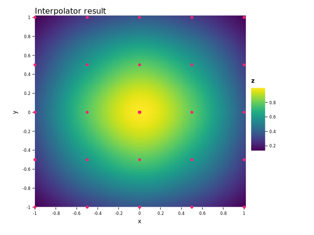
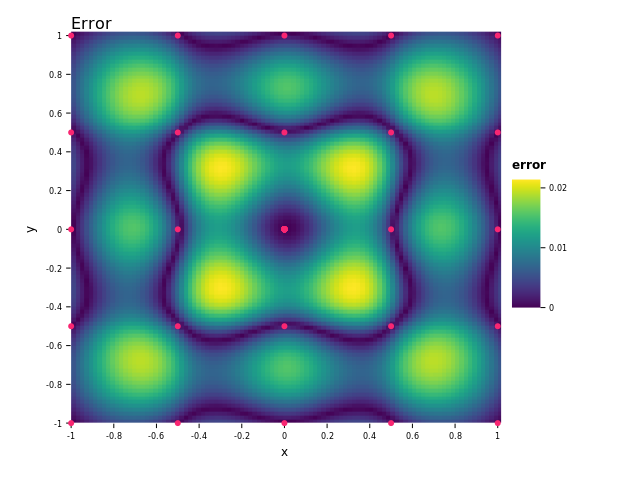
It looks pretty similar to the original function so I'd say it did a good job. We have also plotted the error in the second image. We can see that the interpolant is the most accurate close to the sampled points and the least accurate between them.
ND interpolation
With the addition of Radial basis function (RBF) interpolation, numericalnim now offers an
interpolation method that works for scattered data of arbitrary dimensions.
The conceptual explanation for how RBF interpolation works is that a Gaussian is placed at
each of the data points. These are then each scaled such that the sum of all the Gaussians
pass through all the data points exactly.
Further, the implemented method employs localization using Partition of Unity. This is a method that exploits the fact that a Gaussian decays very quickly. Hence we shouldn't have to take into account points far away from the point we are interested in. So internally a grid structure is created such that points are only affected by their neighbors. This both speeds up the code and also makes it more numerically stable.
The format of the inputs that is expected is the positions as a Tensor of shape (nPoints, nDims)
and the function values (can be multi-valued) of shape (nPoints, nValues). In the general case
the points aren't gridded but if you want to create points on a grid you can do it with the
meshgrid function. It takes in a varargs of Tensor[float], one Tensor for each dimension containing the
grid values in that dimension. An example is:
let x = meshgrid(arraymancer.linspace(-1.0, 1.0, 5), arraymancer.linspace(-1.0, 1.0, 5), arraymancer.linspace(-1.0, 1.0, 5))
echo x[0..10, _]
Tensor[system.float] of shape "[11, 3]" on backend "Cpu" |-1 -1 -1| |-0.5 -1 -1| |0 -1 -1| |0.5 -1 -1| |1 -1 -1| |-1 -0.5 -1| |-0.5 -0.5 -1| |0 -0.5 -1| |0.5 -0.5 -1| |1 -0.5 -1| |-1 0 -1|
which will create a 3D grid with 5 points between -1 and 1 in each of the dimensions.
Now let's define a function we are going to interpolate: $$f(x, y, z) = \sin(x) \sin(y) \sin(z)$$ Here's the code for implementing it:
proc f(x: Tensor[float]): Tensor[float] =
  product(sin(x), axis=1)

let y = f(x)
Now we can construct the interpolator as such:
let interp = newRbf(x, y)Evaluation is done by calling eval with the evaluation point(s):
let xEval = [[0.5, 0.5, 0.5], [0.6, 0.5, 0.3], [0.75, -0.23, 0.46]].toTensor
echo interp.eval(xEval).squeeze
echo f(xEval).squeeze
Tensor[system.float] of shape "[3]" on backend "Cpu"
0.110195 0.0784921 -0.0651828
Tensor[system.float] of shape "[3]" on backend "Cpu"
0.110195 0.0799985 -0.0689888
As we can see by comparing the exact solution with the interpolant, they are pretty close to each other.
Conclusion
As we have seen, you can do all sorts of interpolations in Nim with just a few lines of code. Have a nice day!
Further reading
- numericalnim's documentation on interpolation
- numericalnim's documentation on RBFs
- Curve fitting is a method you can use if you know the parametric form of the function of the data you want to interpolate.